


Interactive performance analysis across weather domains and model architectures, plus supplementary figures and downloadable data referenced in the paper.
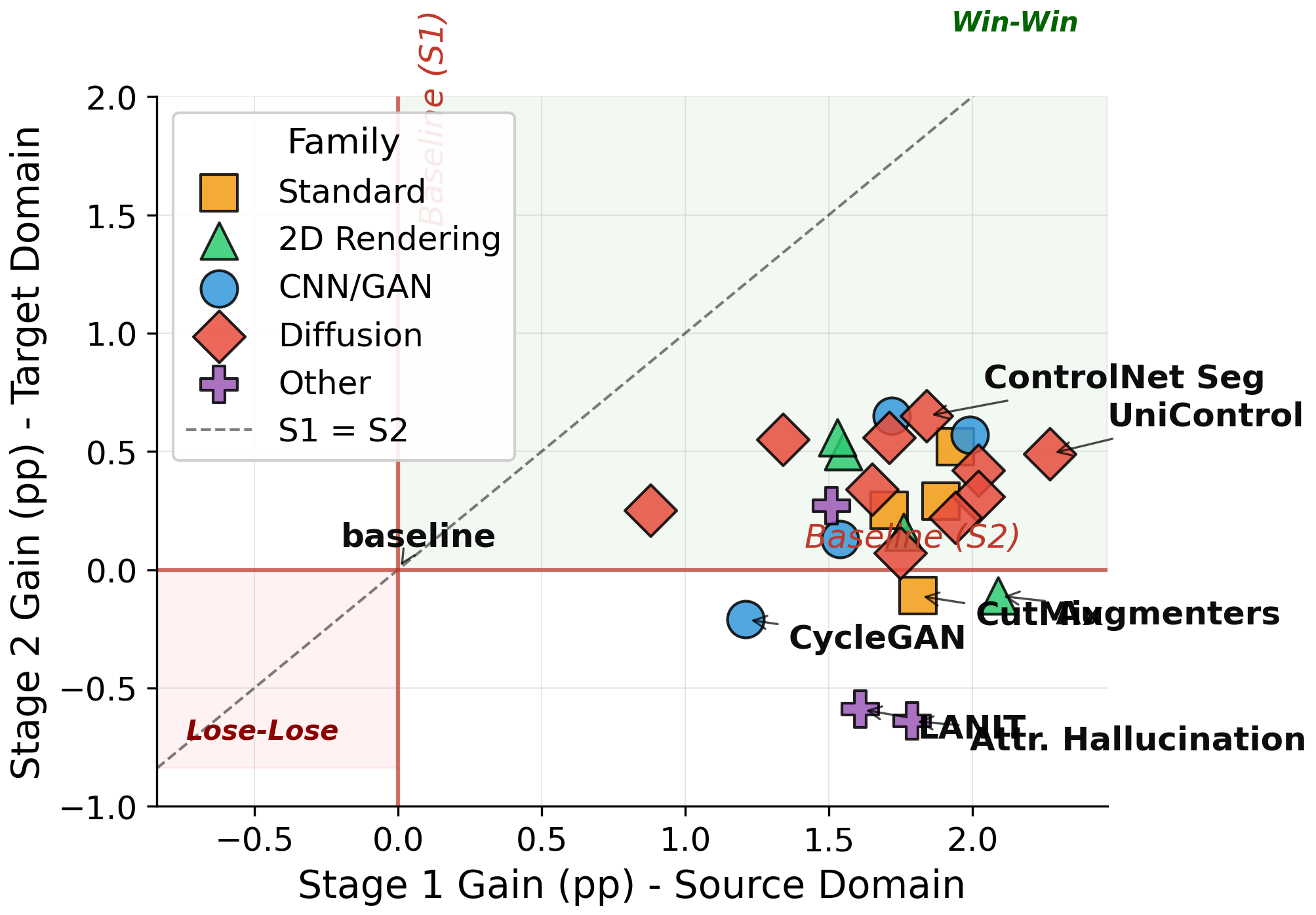
Explore the results interactively. Filter by method family and switch between domain and model views.
Additional figures, detailed breakdowns, and technical appendix content referenced in the paper.
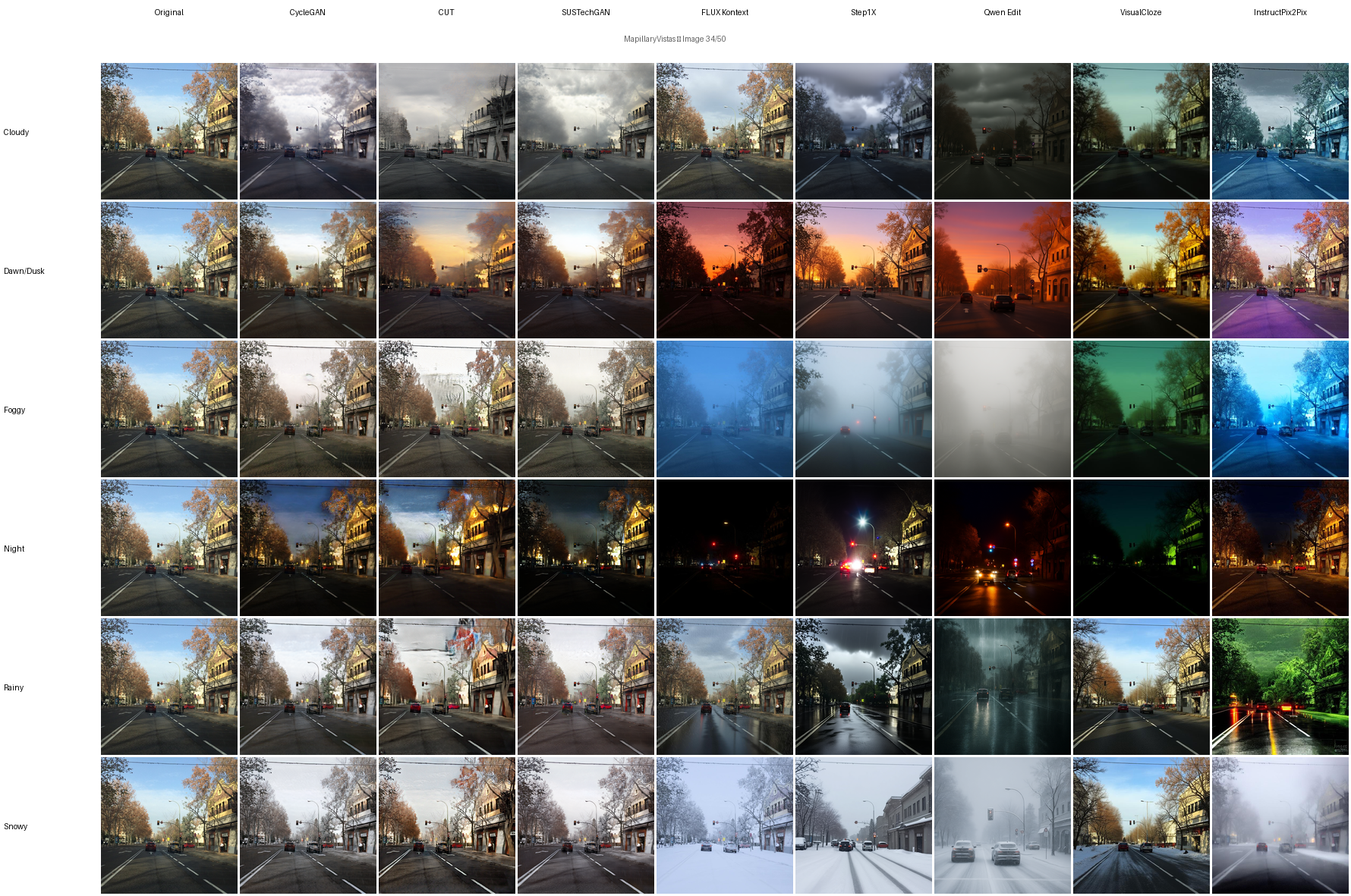
Parametric weather synthesis through classic image processing — no neural networks.
CNN and GAN architectures for unpaired image-to-image translation.
Neural style transfer models for domain-specific appearance manipulation.
Diffusion‐based image-to-image models including ControlNet-conditioned approaches.
VLM and multimodal diffusion models for text-guided weather synthesis.
Standard augmentation pipelines not specific to weather.
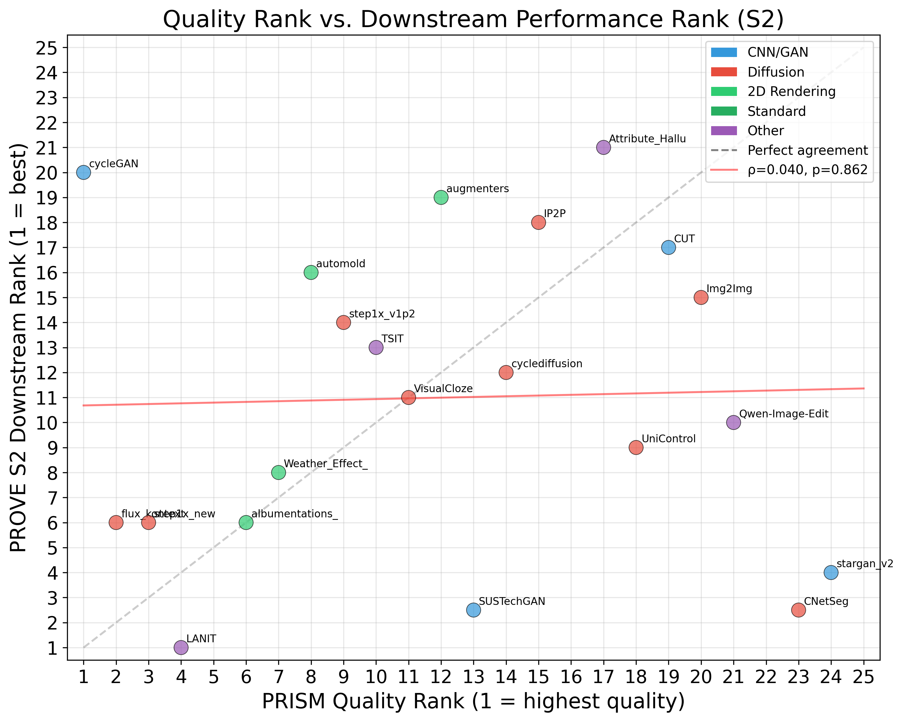
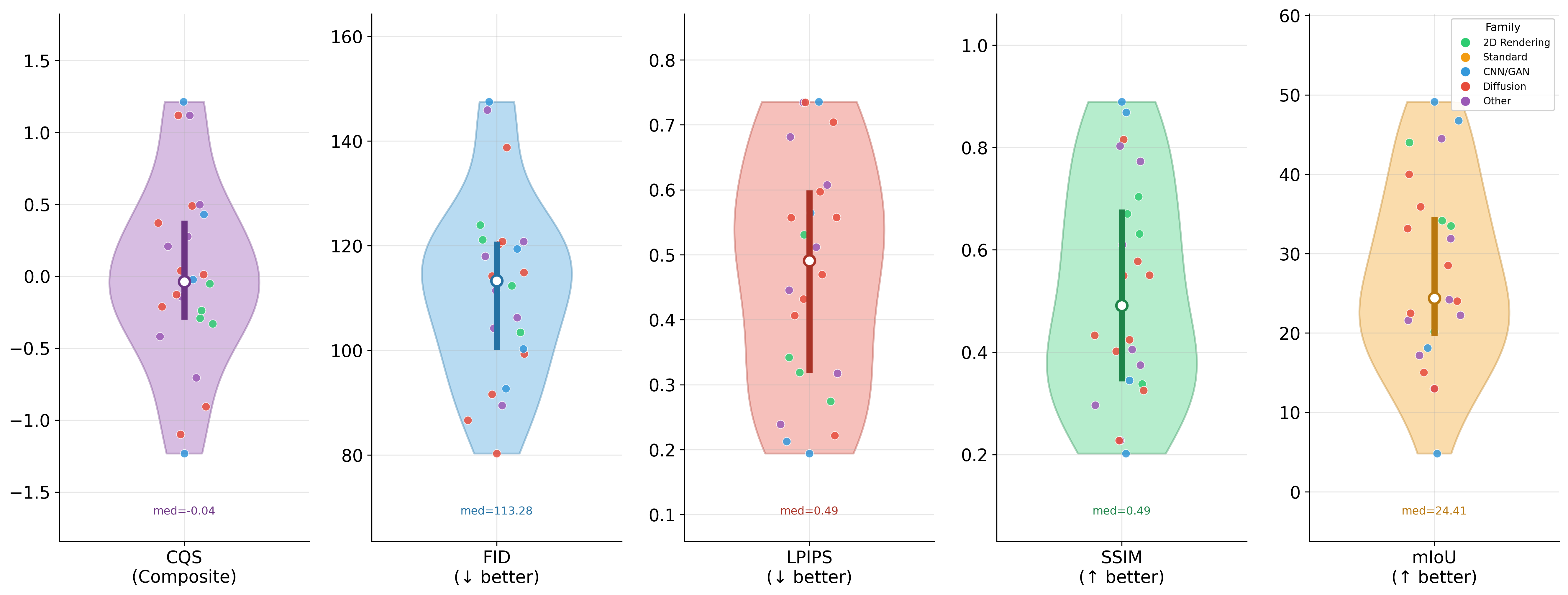
Standardized quality assessment framework computing FID, LPIPS, SSIM, PSNR, pixel accuracy, mIoU, and frequency-weighted IoU for each generative method against original images.
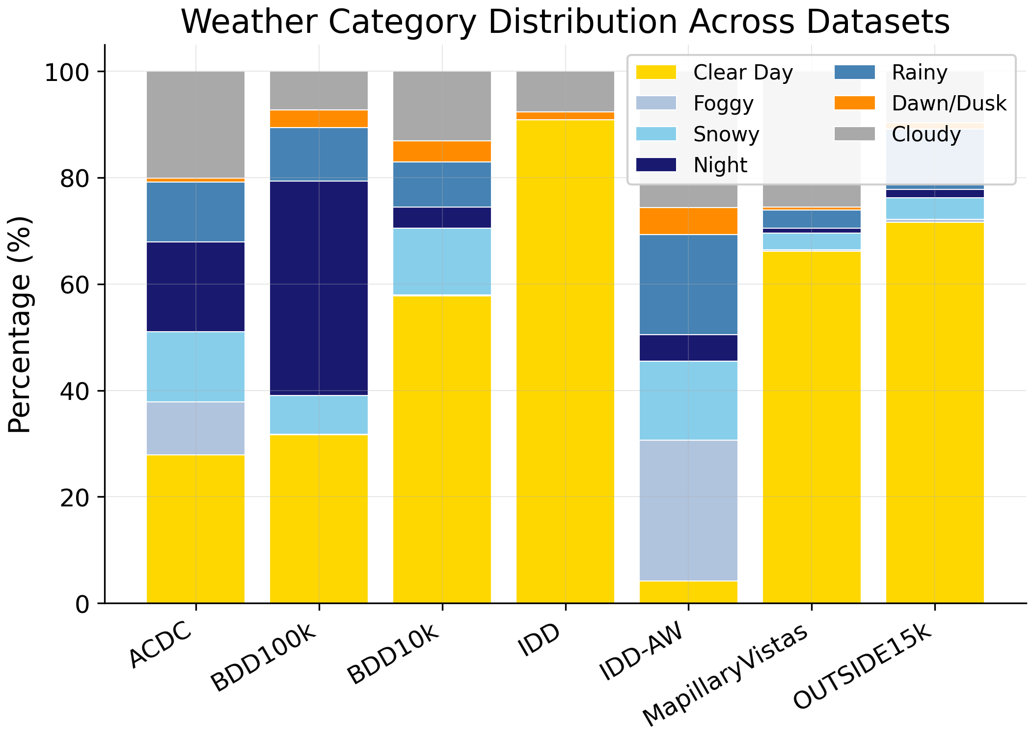
Condition-aware dataset splitting strategy using CLIP-based weather classification. Two-stage process: (1) indoor/outdoor filtering, (2) 7-class weather classification with fog counter-prompts.
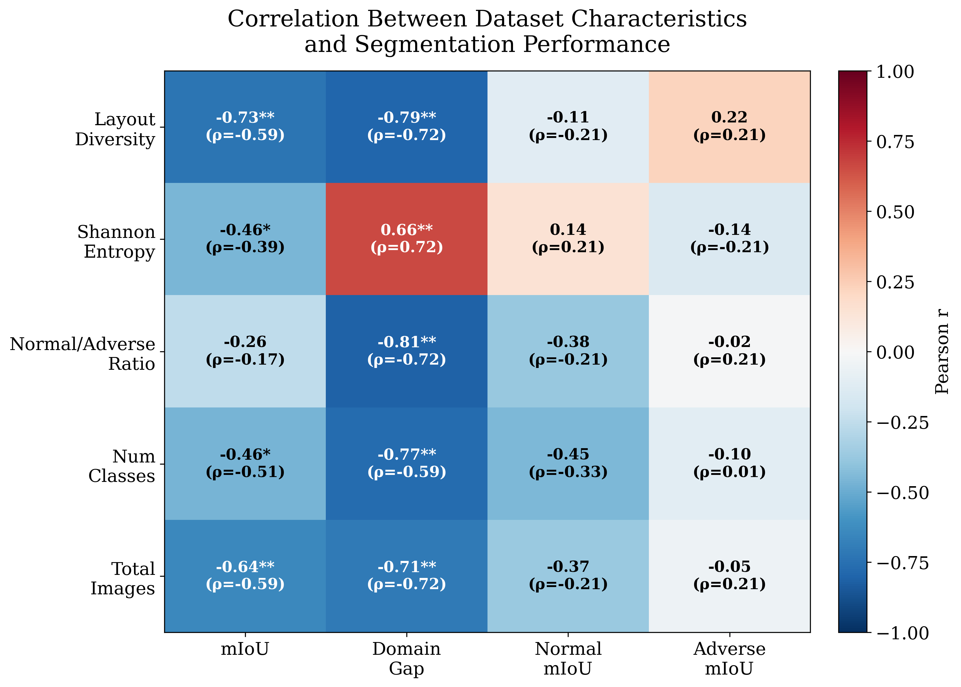
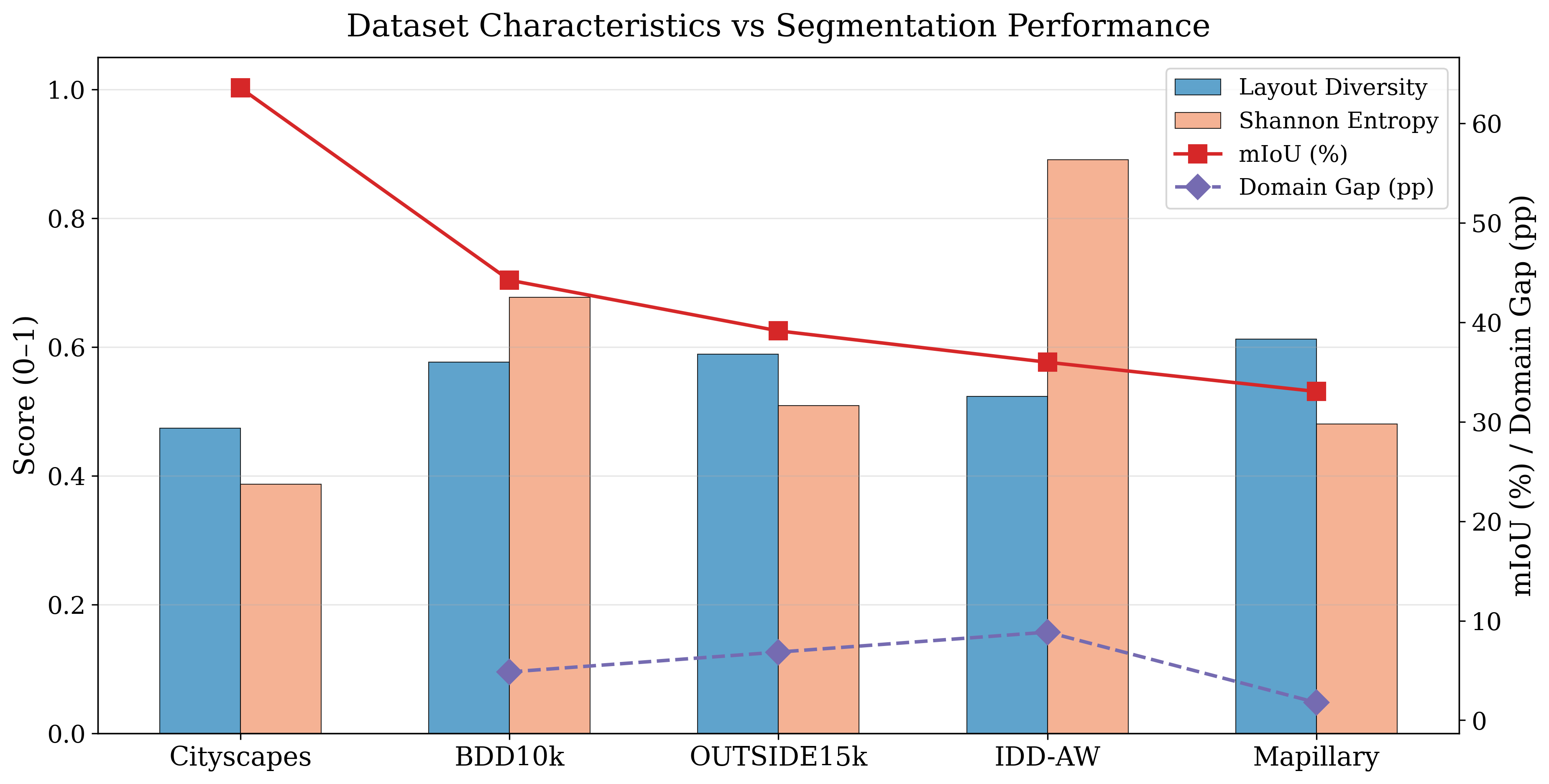
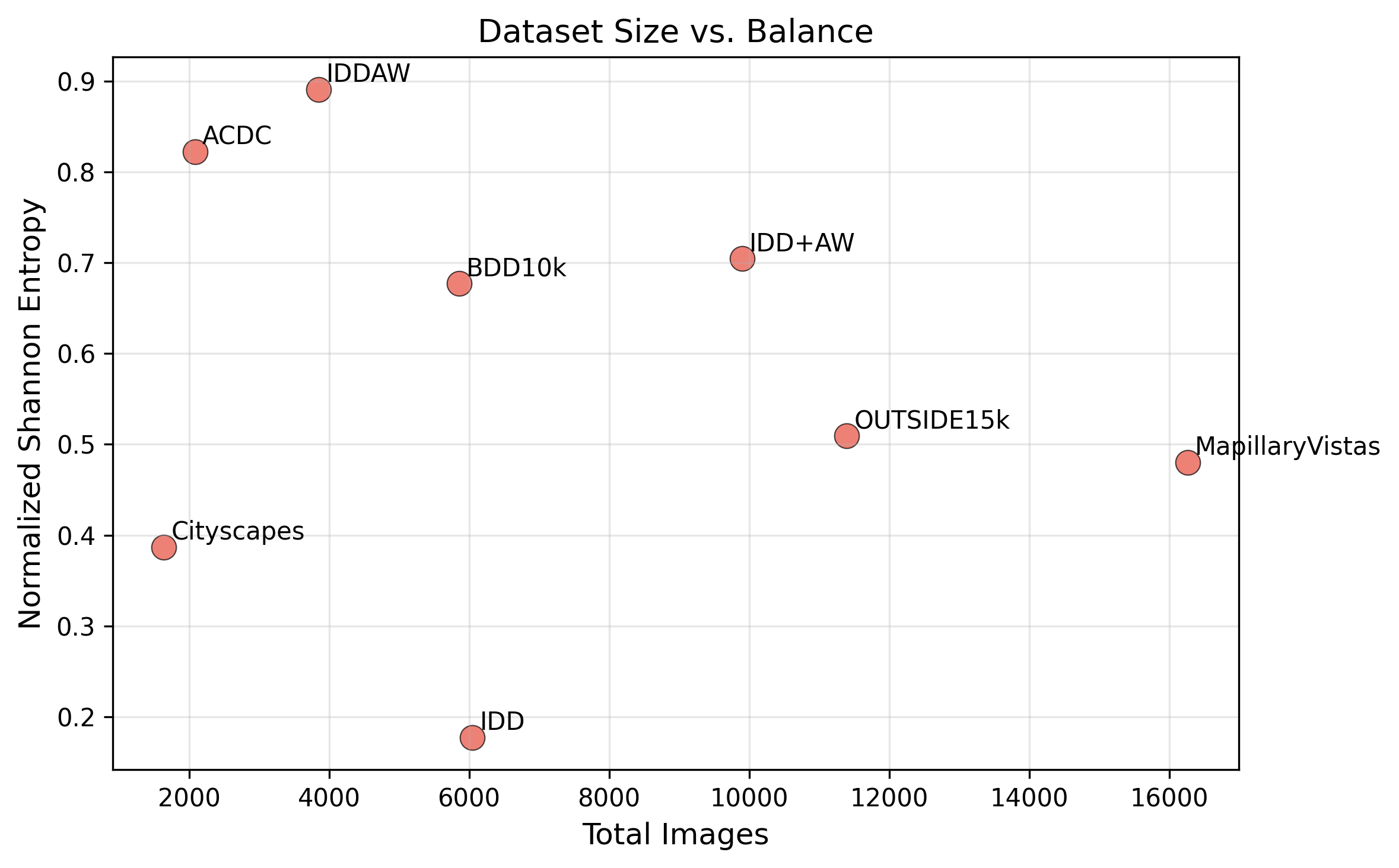
Measures how close a weather domain distribution is to uniform on a 0–1 scale. Used to quantify class imbalance across evaluation datasets.
Normalized Shannon Entropy:
Hnorm = H / Hmax = −Σi=1…K pi ln(pi) / ln(K)
Companion metric — Imbalance Ratio: IR = Nmax / Nmin (ratio of largest to smallest category count).
Pixel-level variant: The same formula applied to segmentation class distributions across pixels, where max entropy uses the count of non-zero classes rather than all possible classes.
Quality thresholds (pixel-level Hnorm):
Measures structural diversity of segmentation layouts across a dataset using Spatial Pyramid Matching (SPM) with Histogram Intersection similarity.
Step 1 — Spatial Pyramid Histograms:
Each segmentation mask is divided into a grid of 2l × 2l cells at level l. Per-cell class histograms are L1-normalized and weighted by level.
Weightl = 0.5(Lmax − l + 1) where Lmax = 3
Step 2 — Descriptor & Similarity:
Descriptork = ⊕l∈levels wl · SpatialHistogram(Mk, l)
Similarity(i, j) = Σd min(Descriptori[d], Descriptorj[d])
Step 3 — Diversity Score:
Diversity = 1 − mean(Similarityoff-diagonal)
Benchmark parameters:
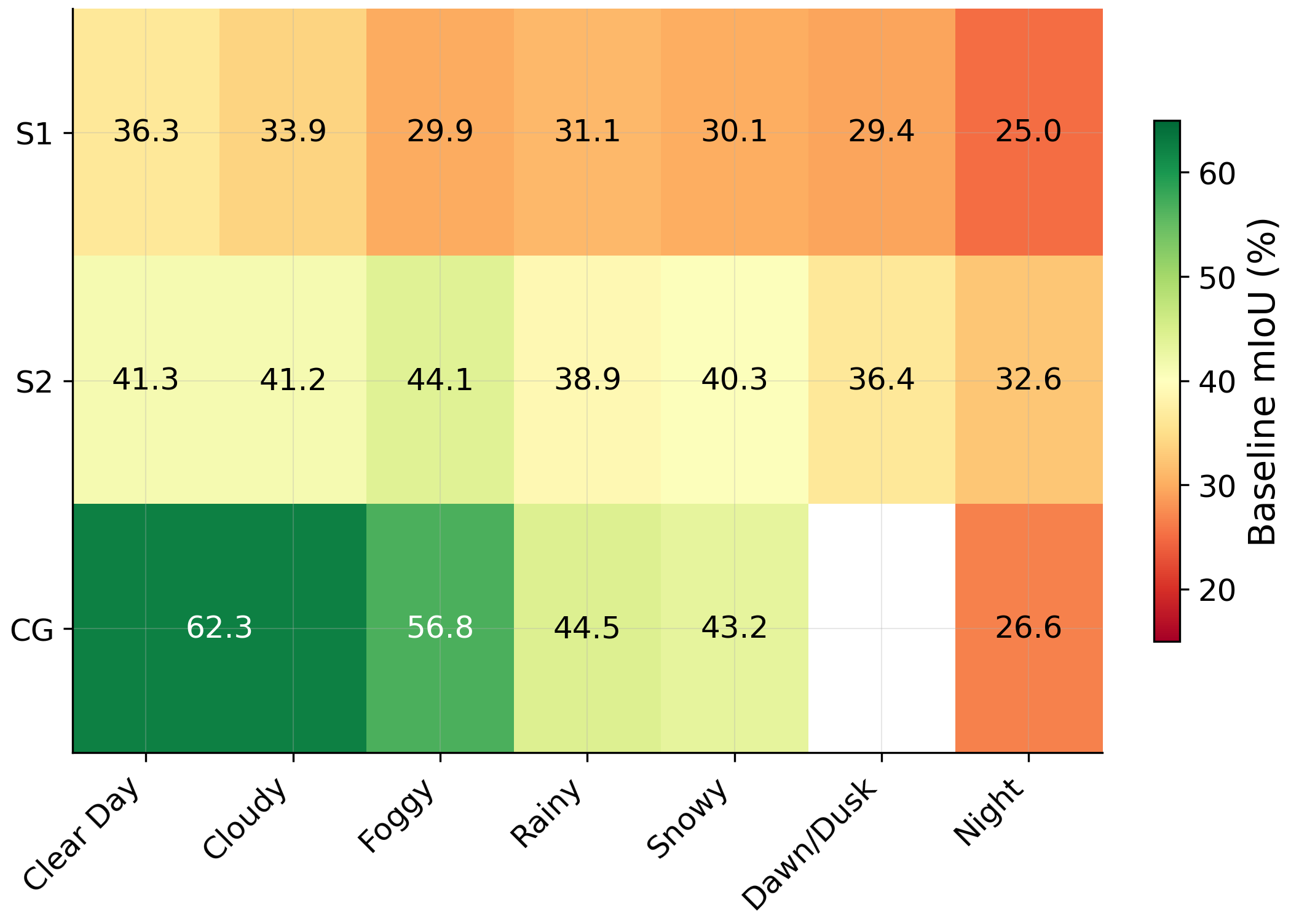
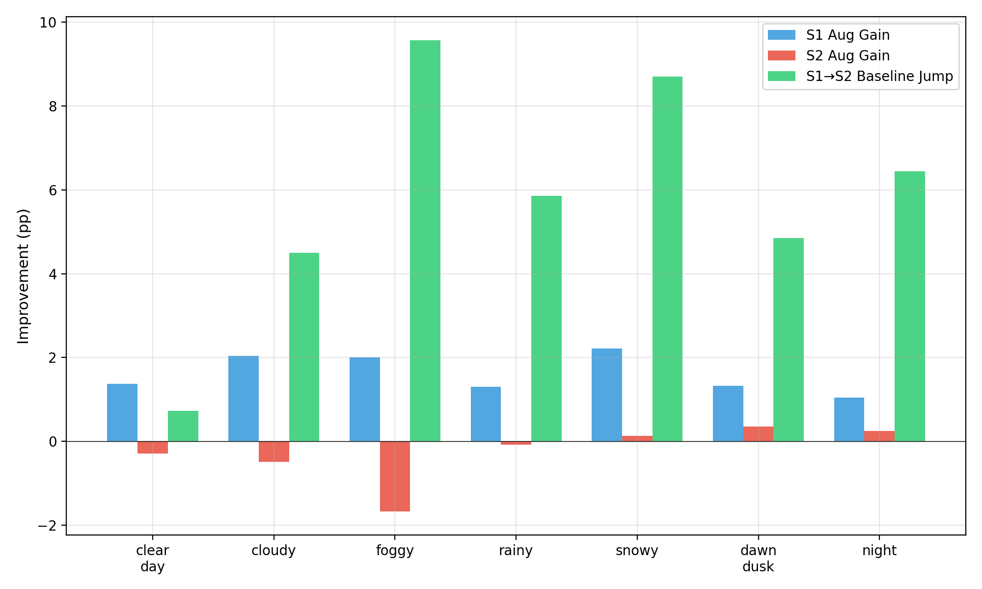
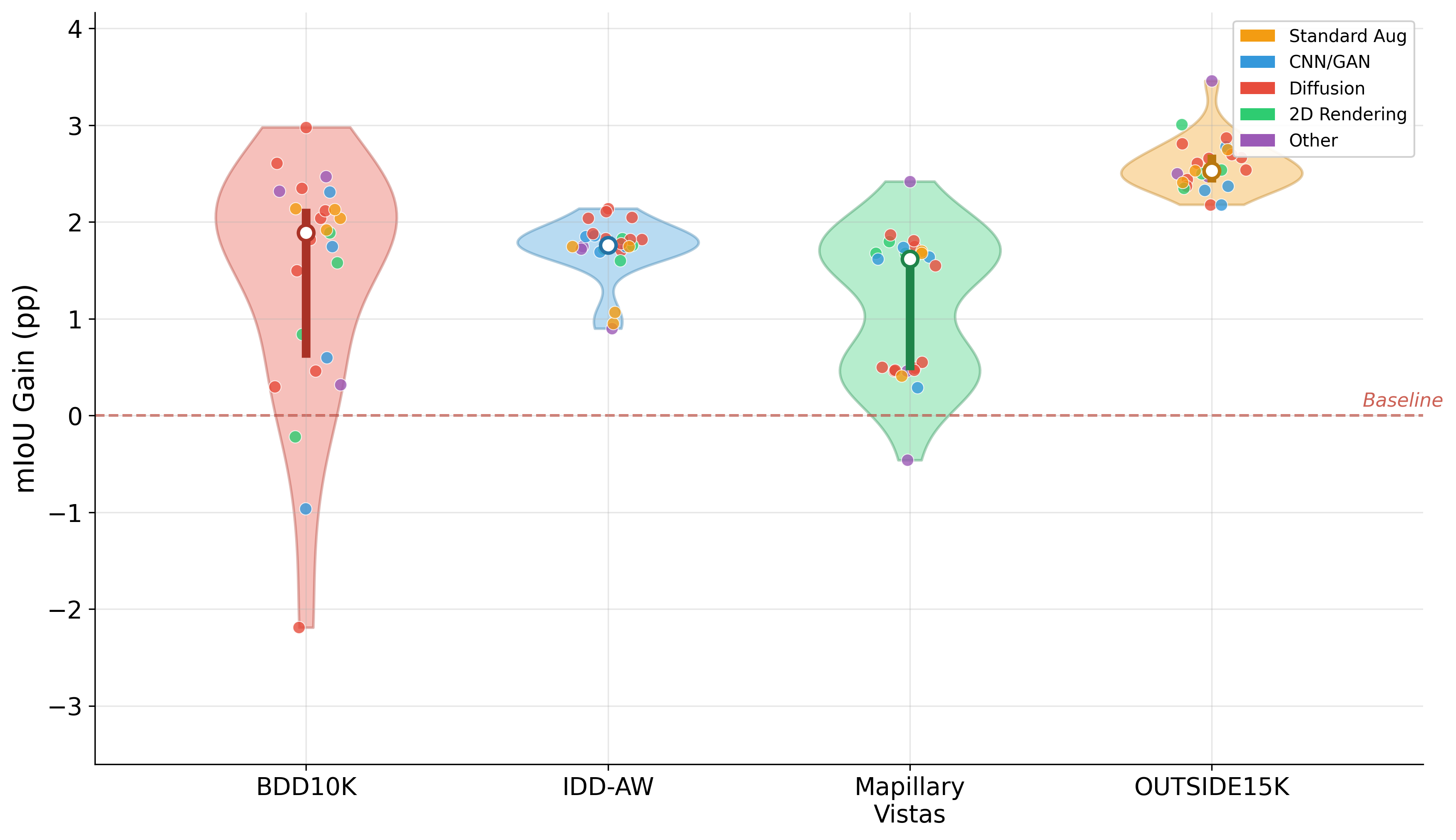
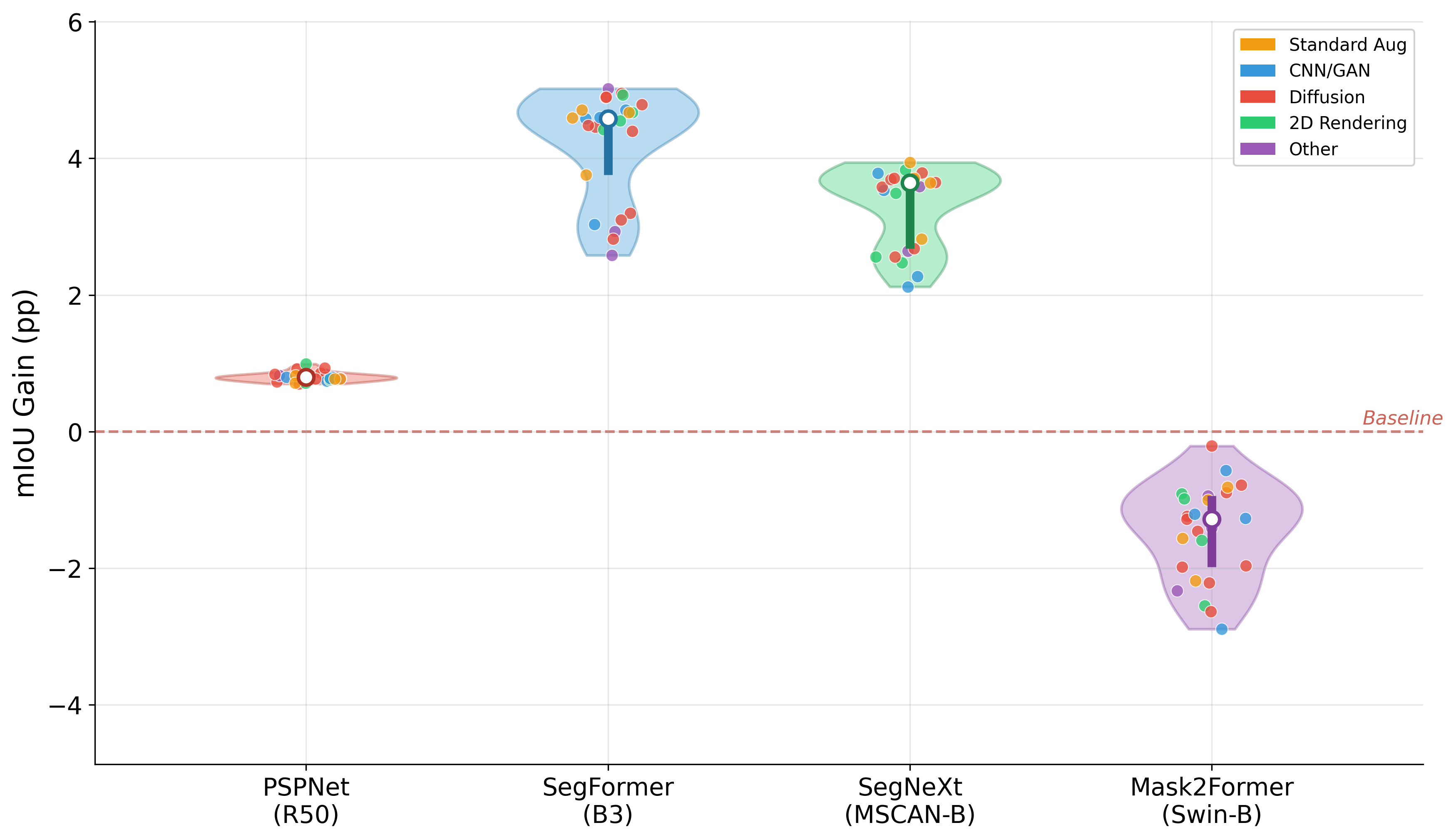
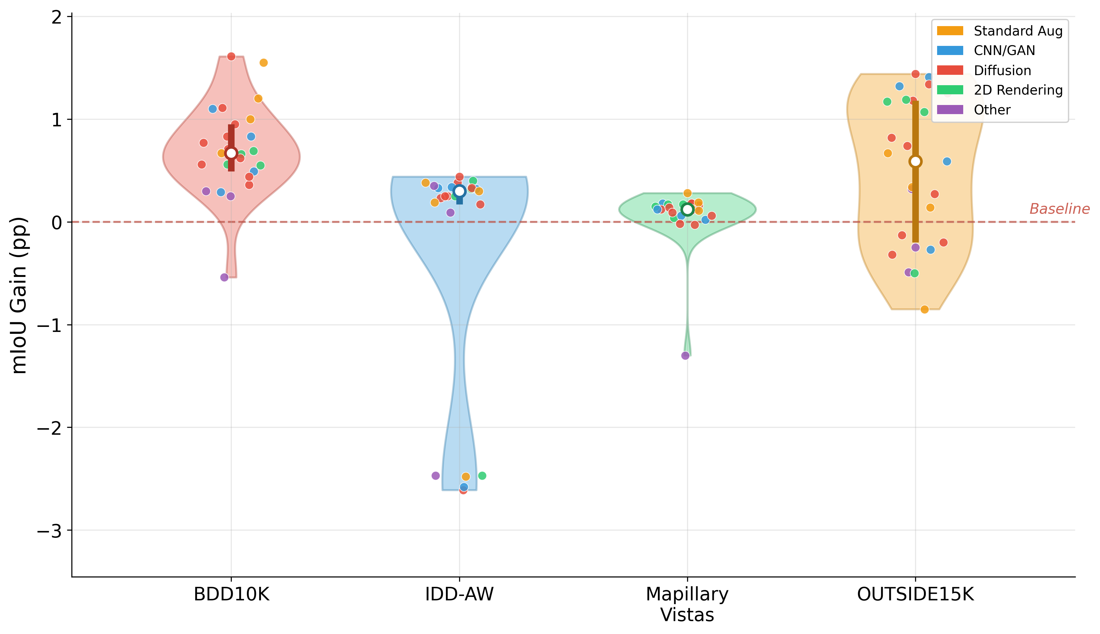
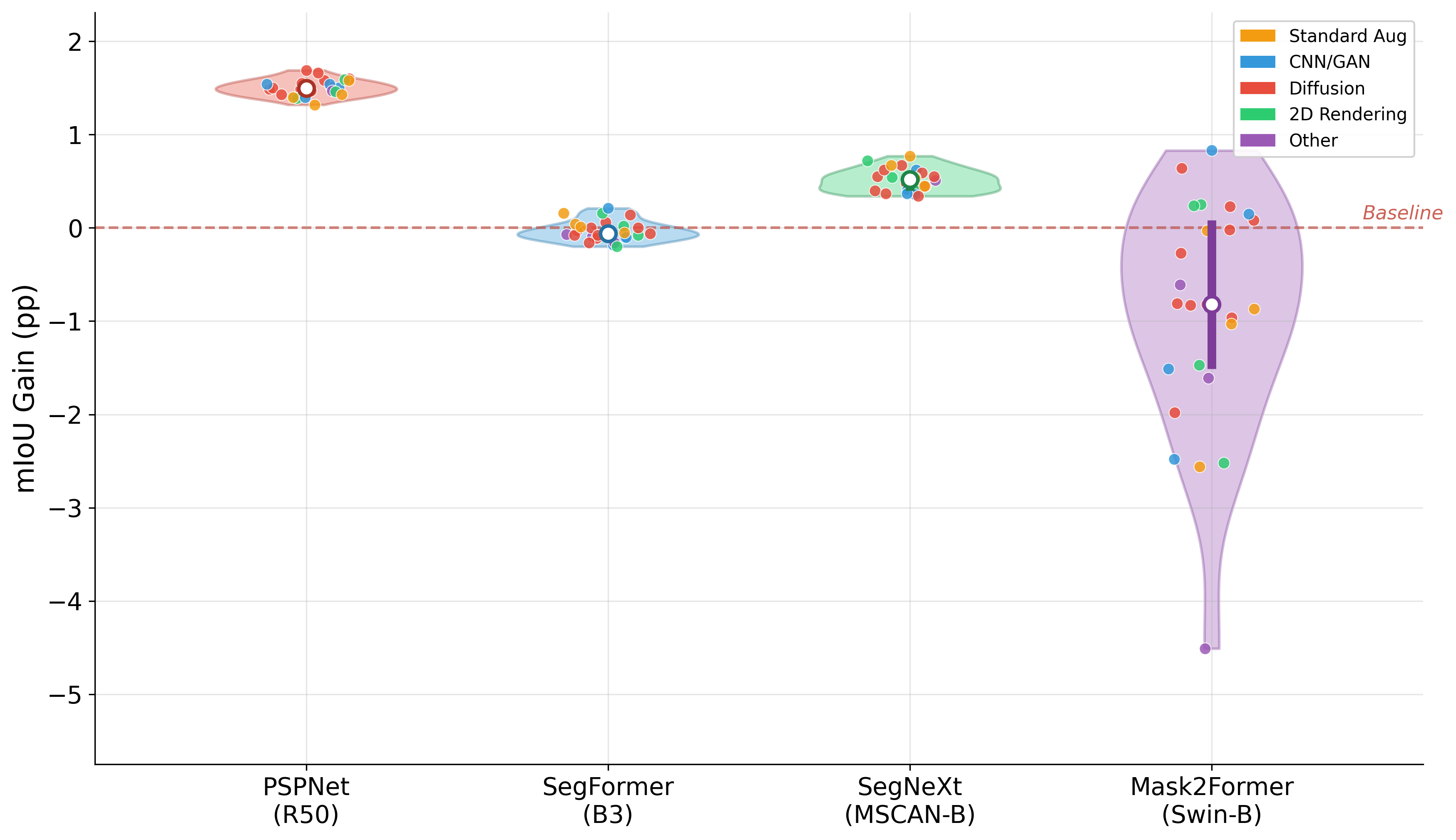
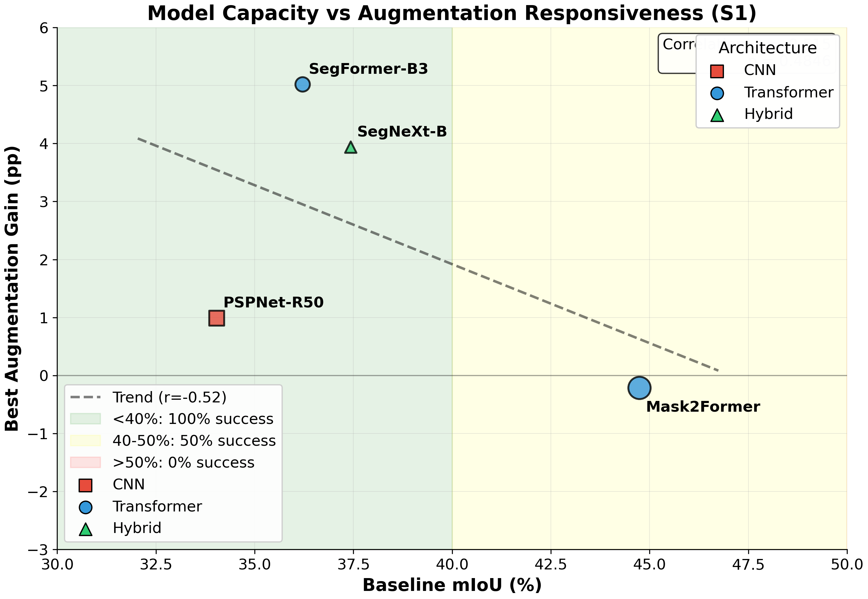
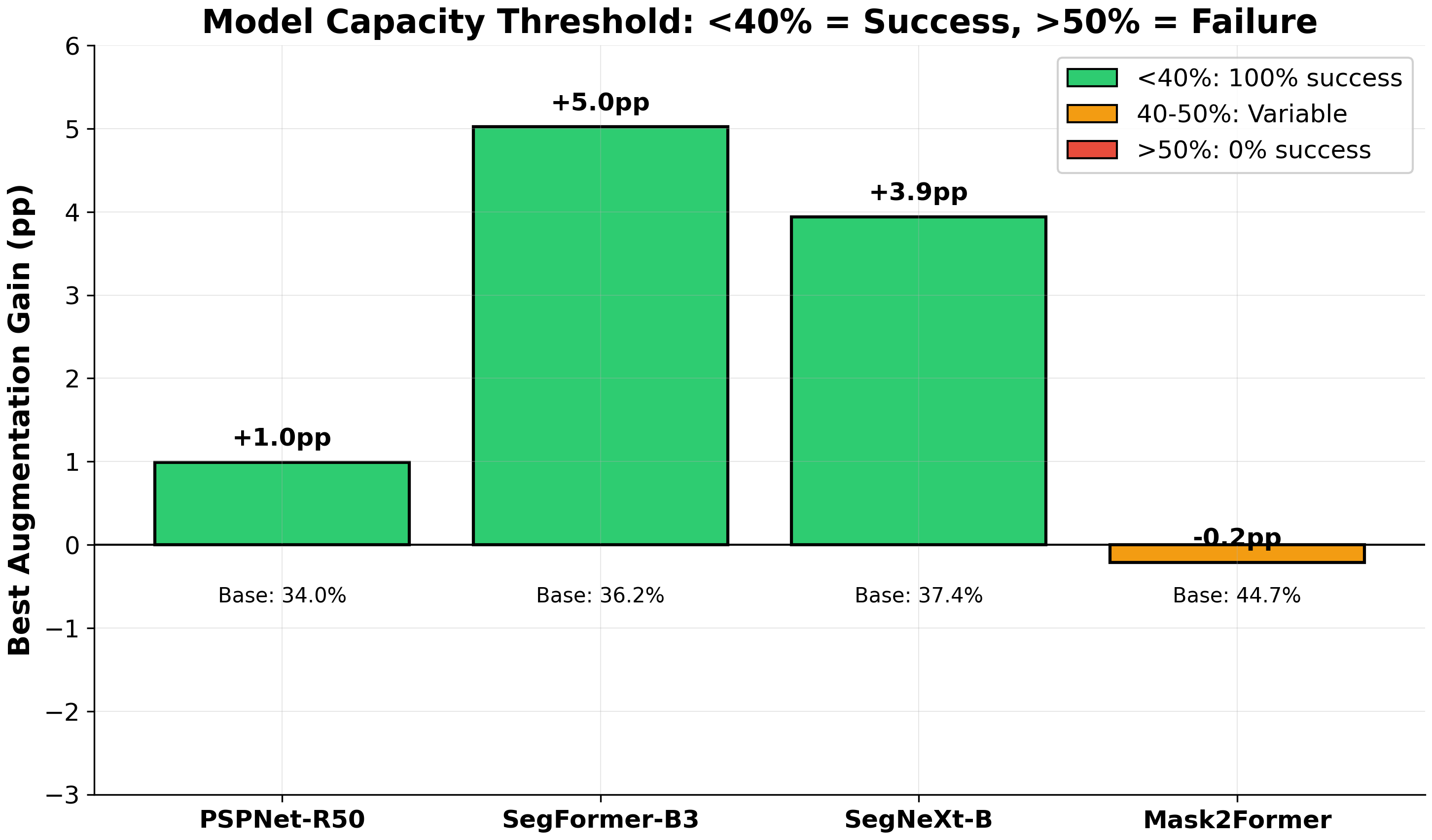
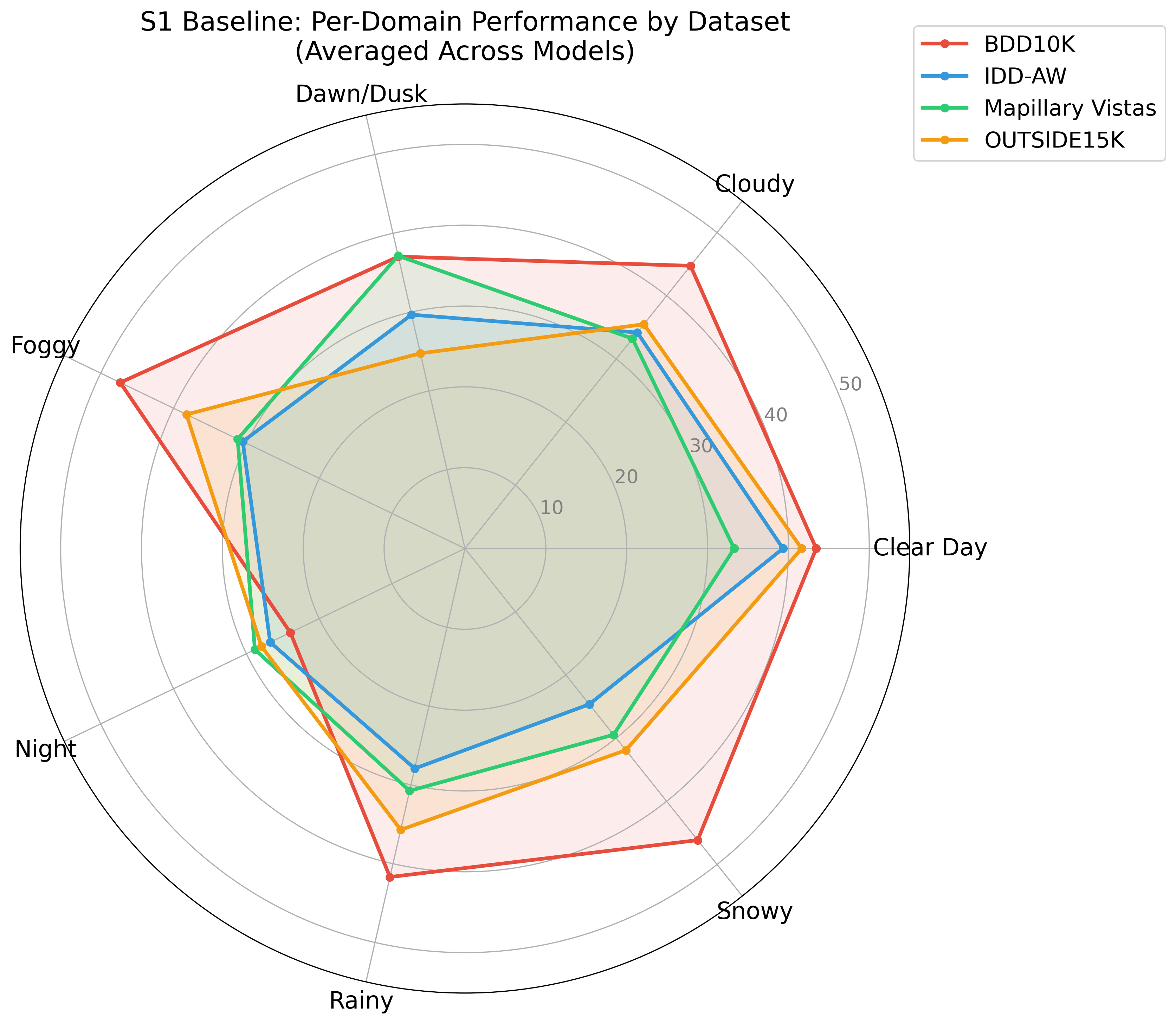
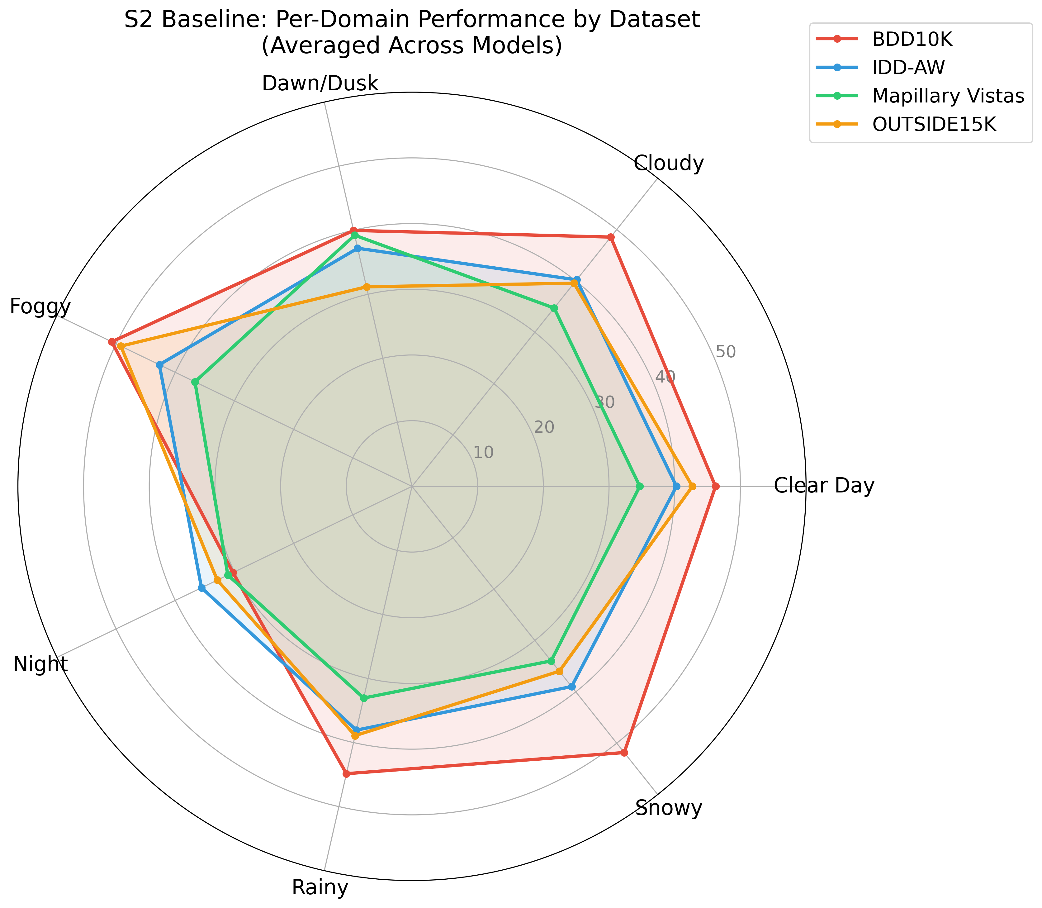
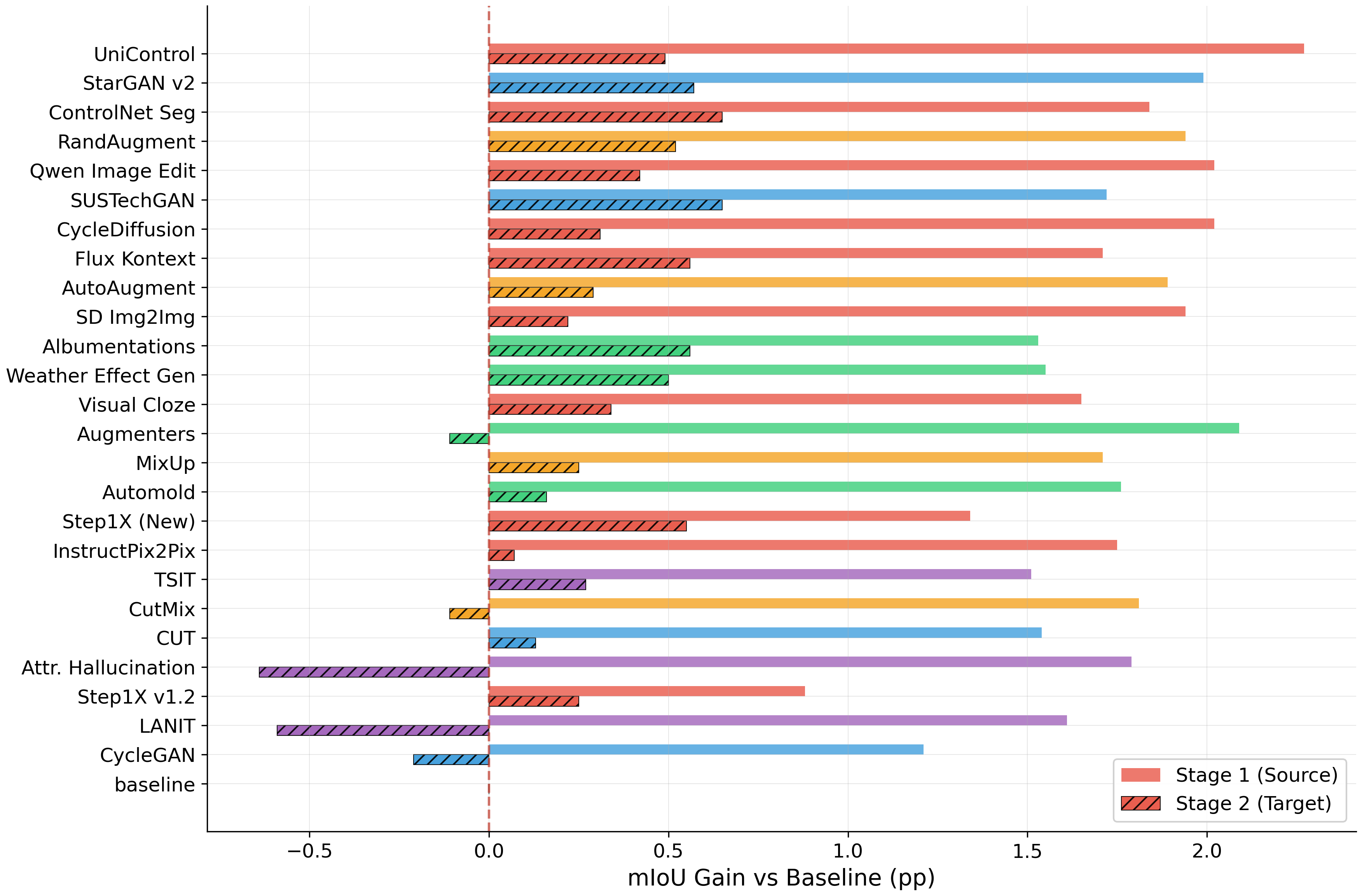
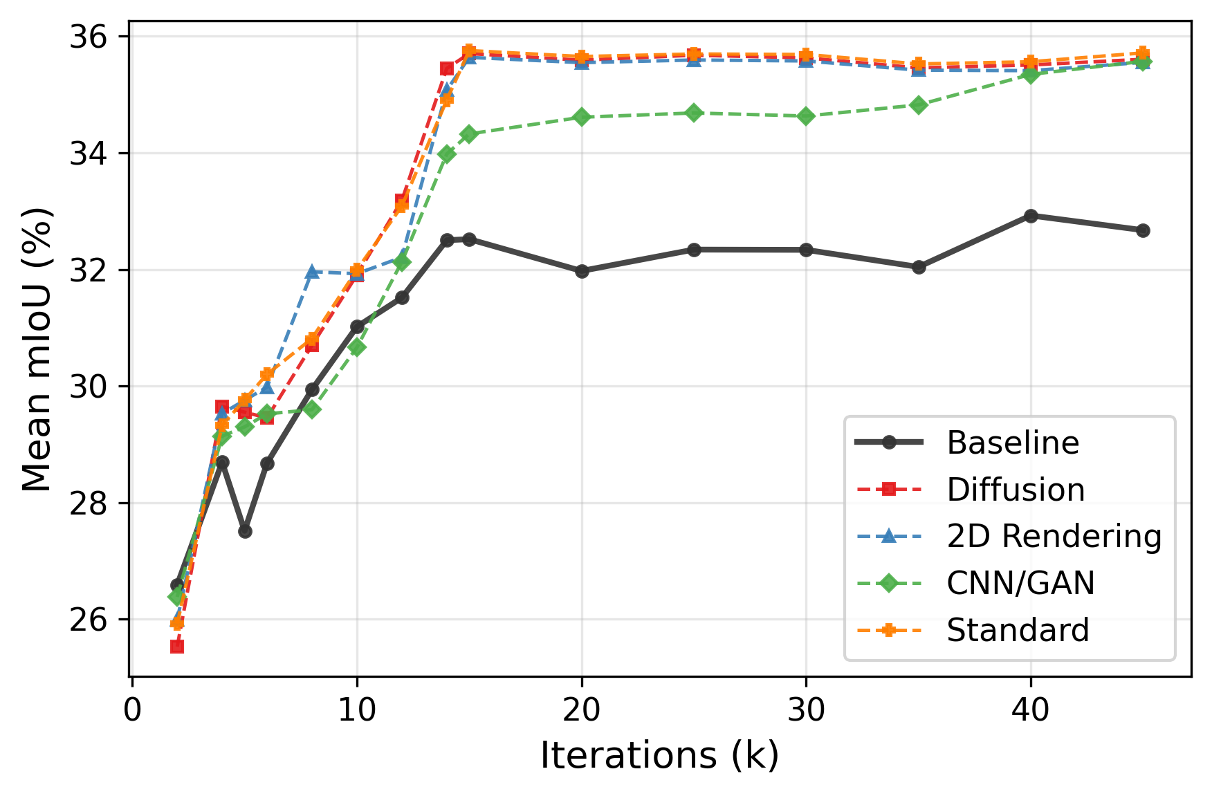
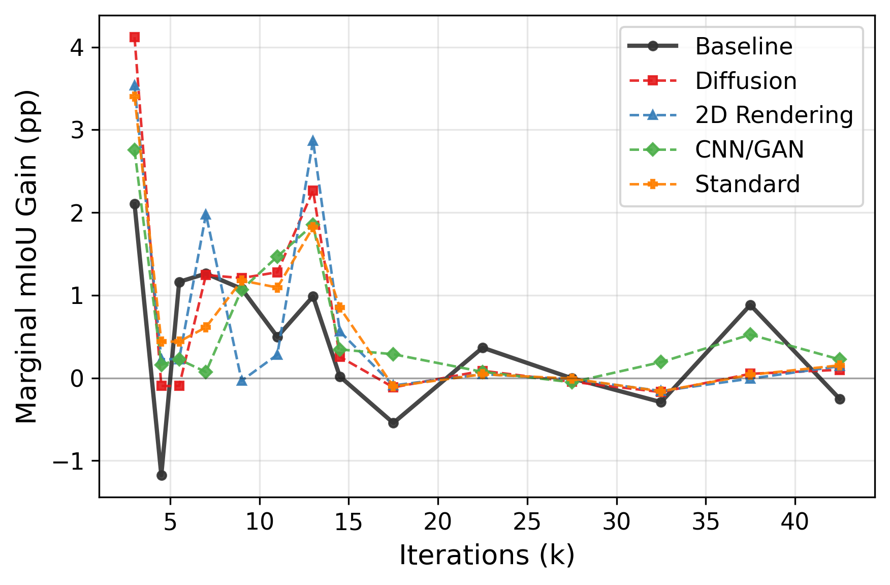
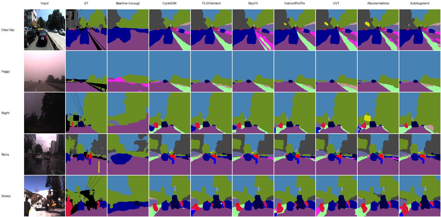
Systematic downstream evaluation framework. Tests each augmentation strategy across all model × dataset combinations, computing per-domain and aggregate performance metrics.